Characteristics of Domestic Cross-Metropolitan Migrants

Domestic migration across U.S. metropolitan areas is selective: in-migrants to expensive metros tend to have higher incomes and educational attainment than out-migrants, while the opposite is true in the least expensive metros. This pattern contributes to the process of polarization across U.S. metros. It also helps sustain expensive metros’ housing price appreciation above and beyond any rise in incomes.
In-migrants to expensive metros tend to have more earners per household, be younger and less likely to own a home than out-migrants. This pattern suggests the notion of a transient class: individuals who arrive in expensive metros as young adults, but are priced out and leave at the point of raising children.
Possible implications of sustained housing price appreciation are discussed briefly with respect to a new class distinction between owners and renters, and with respect to the long-run security of expensive coastal metros’ leading role.
Since the 1970s, the cost of housing in U.S. metropolitan areas has sharply diverged. Some metros, typically in the Rust Belt, saw their economic base decline and their housing needs met or even exceeded by the existing housing stock, which has resulted in cheap homes. In contrast, metros with healthy economies kept attracting people, generating demand for housing. When such demand was met by abundant new construction in sprawling suburbs, as tended to happen in the South, populations grew and housing affordability was maintained. But in the coastal metros, where sprawl was subdued and the development of new housing severely diminished, the demand for housing fueled home price appreciation instead of population growth.
Apart from making the coastal cities more expensive, these circumstances also altered the selection of people moving between U.S. metro areas. In other words, instead of just affecting how many people moved between places, they also affected who those people were. This study sheds light on the latter.
Income
The chart below looks at income. It plots the difference between each metro’s in- and out-migrants’ incomes, and how these differences vary between metros depending on how expensive they are. The San Francisco Bay Area is the nation’s most expensive metro area, and is located in the top right corner. Its position above the red line indicates that, on average from 2005 to 2016, in-migrants to the San Francisco metro earned $12,640 a year more per household after arriving than out-migrants did before they left (see Data and Methodology section for details).
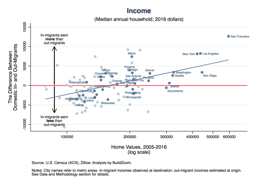
San Francisco demonstrates an extreme version of a selective migration pattern that I call positive income sorting. But even if we disregard it as an outlier, the pattern across metros is clear: the difference between in- and out-migrants’ incomes is more positive in cities with higher housing prices, and vice versa. This doesn’t mean that a metro with positive income sorting only sees high-income households moving in and low-income households moving out. What actually happens is that households of all income levels move in and out of every metro area. Even the most expensive metros see substantial numbers of low-income households moving in, but the incomes of their in-migrants skew higher and those of their out-migrants skew lower, as reflected the medians of these flows.
In addition to the San Francisco metro area, other expensive coastal metros such as Los Angeles and New York also exhibit positive income sorting. In- and out-migrants in lower-priced metros like Atlanta and Dallas appear to have similar incomes. Rust Belt metros like Cleveland and Detroit exhibit negative income sorting, whereby the median household moving in earns less than the one moving out.
Download metro-specific numbers for all metro areasWhy do the expensive coastal metros exhibit positive income sorting? These metros are expensive because they have restricted their supply of new housing even as they continue to generate strong demand for it. As a result, homebuyers and renters in these metros compete with each other over a smaller housing stock, bidding up prices, and pushing out those who are the least financially able. The high cost of housing also deters potential in-migrants, especially if their incomes are low, which drives up the income levels of those who are ultimately observed moving in. Of course, homeowners and certain fortunate renters can stay put in their homes for a long time, even when they can no longer afford them at current prices, so positive income sorting can be a slow process.
Earners Per Household
Besides having a higher income, in-migrants to expensive metros also tend to have more earners per household than out-migrants (for both groups, the number of earners per household is observed at the destination). The difference reflects a greater prevalence among in-migrants of dual-earner couples and of households comprised of roommates. Indeed, those moving from low-cost places to more expensive ones are likelier to need multiple incomes to make ends meet.

But that is only part of the story. In addition to requiring multiple incomes of newcomers, the high cost of housing in expensive metros often compels households with fewer earners, such as single-parent families, to leave. In other cases, individuals live in multiple-incomes households out of necessity, even though they would rather not. Such individuals may be compelled to leave expensive metros if doing so would allow them to live without roommates, or if it would allow a parent to stay home with the children. The Sacramento metro area, for example, has fewer earners per household among its in-migrants than its out-migrants, and that is probably not a coincidence because it is a key destination of those leaving the San Francisco Bay Area in search of cheaper housing.
Age
In the most expensive metros, in-migrants tend to be younger than out-migrants. In the least expensive metros it is the opposite.

The pattern observed with respect to migrants’ age is consistent with the notion of a transient class, whereby individuals arrive in young adulthood to experience the life and career opportunities that expensive metros have to offer, and leave once they confront the realities of raising children in this environment. The notion of a transient class is also consistent with the pattern observed earlier with respect to the number of earners per household, especially inasmuch as it is driven by expensive metro in-migrants boarding with roommates, and families with children seeking cheaper housing elsewhere.
Fast-forwarding to a later chapter in life, the Miami, Orlando, Tampa and Phoenix metro areas stand out as retirement hubs. In-migrants to these metros tend to be substantially older than out-migrants. The fitted blue line in the graph indicates the average relationship between the in- and out-migrant age difference and metros’ housing price levels, and indeed these metros are located well above the line, indicating that their in and out-migrant age differences are more positive than their housing price levels would suggest. In-migrants to these metros also tend to have higher incomes and fewer earners per household than out-migrants–as well as higher owner-occupancy rates, as we will see in a moment–all consistent with their role as retirement hubs.
Owner-Occupancy
In-migrants arriving in expensive metro areas are less likely to become owner-occupants than out-migrants (out-migrants owner-occupancy status is observed at the destination; it is unobserved at the origin, unfortunately). Not only is it harder for in-migrants to buy a home when housing is expensive, it is also enticing homeowners in expensive metros to monetize their property and head to cheaper parts of the country, where they typically buy a home.

Education
Perhaps the most important chart in the sequence is the final one, below. It shows in more expensive metros, in-migrants tend to be more educated than out-migrants, and vice versa, i.e. that there is positive sorting along education lines. It is already the case that the nation’s most expensive metros have more educated populations. The fact that migration helps raise overall education levels in the more expensive metros while lowering them in less expensive ones only helps widen the existing rift.

This pattern is particularly concerning for metros whose in-migrants are less educated than out-migrants, because it does not bode well for their ability to cultivate a knowledge-based economy. One facet of the problem is that, compared to their less educated neighbors, these metros’ more educated residents are more inclined to move to expensive metros and face less difficulty in doing so. The quality of an institution like Carnegie-Mellon and its implications for its graduates’ ease of moving elsewhere, for example, could help explain why the difference between in- and out-migrants’ education levels in the Pittsburgh metro area has been negative.
Polarization, Housing, And The Industrial Mix
Positive income sorting and the role of migration in widening the educational gap between metros jointly amount to directly observing polarization–the process whereby America’s metropolitan areas grow increasingly dissimilar along socio-economic dimensions. Given the current political scene in the U.S., the importance of polarization goes without saying.
The housing market is closely intertwined with the process of polarization. Because income and educational attainment are highly correlated, positive income sorting means that those who move into expensive metros tend to be more educated, and those who leave them less so.
But statistical analysis of the underlying data suggests that polarization is rooted in more than just the housing market, and also derives from other differences between metropolitan economies (the analysis is presented in the Data and Methodology section ). The fluctuations of housing prices from year to year within each metro correspond to changes in the difference between in- and out-migrants’ owner-occupancy levels, as well as the number of earners per household. This means that people, including in- and out-migrants, react when housing prices rise and fall by adjusting their decisions vis-a-vis working, and with respect to homeownership, rentership and living with roommates. In contrast, differences between in- and out-migrants’ income and educational attainment levels do not vary from year to year in sync with housing price fluctuations. Rather, the intensity of sorting between metros along income and education lines corresponds only to differences in housing price levels across metro areas, but not to each metro’s own year-to-year fluctuations. This suggests that, in addition to any role that housing market conditions play with respect to polarization, there are other facets of metropolitan economies that underlie polarization as well.
Metro areas’ industrial mix, for example, is closely related to residents’ education and to the incomes they command, but its influence on migration patterns does not fluctuate from year to year in tandem with housing prices. America’s coastal metros are expensive not just because their natural geography and land use policies restrict the housing supply, but also because their industrial mix skews towards knowledge-centric sectors. These sectors’ growth contributes to the demand for housing, as do the wages earned by their educated workforce. Indeed, the concentration of such industries in the expensive coastal metros helps explain why we observe positive sorting into these metros along income and education lines in the first place. But, crucially, their concentration also explains why the intensity of this sorting does not correspond to housing price fluctuations from year to year.
Although the industrial mix is slow to change and does not noticeably respond to housing price fluctuations from year to year, housing prices can help shape the industrial mix over extended periods time. By affecting who can afford to live in the metro area, the cost of housing helps determines the feasibility of different industries’ and employers’ presence there. Employers that rely on low-wage labor for producing tradable goods and services have all but vanished from the expensive coastal cities, and would be at a huge disadvantage if they located there today. On the other hand, employers who require low-wage labor for non-tradables, such as restaurants and hotels, must either pay higher wages or suffer the consequences of labor shortage.
Positive Income Sorting Helps Sustain Housing Price Appreciation
“Who can afford to live here and for how long?” is a question often raised by residents in expensive metros. Indeed, as the housing cycles approach their peak and the discrepancy between rising home prices and sluggish earnings growth is most apparent, that question may seem to pop up in every conversation.
Positive income sorting in the nation’s most expensive metros helps sustain housing price appreciation. Of course, if current residents’ income rises that helps sustain price appreciation, but sustained appreciation does not require a proportional increase in current residents’ income. Instead, positive income sorting helps the population afford housing at higher prices by substituting out-migrants with more financially-able in-migrants. If those leaving would have stayed had housing prices not risen as much, then the process of positive income sorting can rightfully be called displacement.
Positive income sorting also calls into question whether comparing home prices to residents’ incomes to determine metro areas’ “affordability” is always a meaningful exercise. When housing price appreciation in a metro is sustained by swapping out low-income residents for higher-earning ones, can statements about “affordability” be taken at face value?
Owner and Renter Class Distinctions
Income and wealth are not the same. When growth in home values outpaces income growth (including due to sorting), buying a home comes to depend more heavily on wealth than on income. Thus, if sustained housing price growth in the expensive coastal metros exceeds the pace of income growth for an extended period, this could cause homeownership to become more dependent on cross-generational assistance and less dependent on within-generation income. This state of affairs would sharpen the distinction between owners and renters, aligning them more closely with socio-economic class than with people’s stage in the life cycle. It would also be consistent with a young, transient class of high-income, low-wealth individuals and households that find it difficult to put down roots in these metros.
Sowing The Seeds For New Metros To Take The Lead
Sustained housing price appreciation could also exert increasingly selective pressure on the kinds of jobs that are feasible to maintain in the expensive metros. Employers who wish to stay in business cannot afford to pay workers a wage that exceeds their contribution to revenue. As a result, employers in the expensive coastal metros would be compelled to maintain only the most productive roles–those which justify wages high enough to compensate for local housing costs–and other types of work would either be foregone, automated, or relocated.
The expensive coastal metros currently lead the U.S. economy. Although the most crucial roles in these cities would be the last to go anywhere, sustained housing price appreciation could nevertheless threaten these metros’ standing. As housing costs increase, the productivity threshold beneath which jobs could no longer remain in these metros would gradually rise, sending workers from ever-higher up the value chain to concentrate elsewhere. As a result, other metro areas’ odds of achieving critical mass for viable new industrial clusters would rise, and ultimately threaten the expensive coastal metros’ lead.
The expensive coastal metros could avoid this scenario by providing sufficient new housing to curb housing price appreciation. It is ironic that these metros are risking their economic future by not doing so, only for the sake of protecting incumbent homeowners from change.
Data and Methodology
Data: this study uses data from the American Community Survey (ACS) and from the Zillow Home Value Index. In particular, it relies on individual- and household-level data from the 2005-2016 1-year ACS files, and on county-level ZHVI data.
Definition of metropolitan areas: in order to avoid conflating migration between a narrowly defined metro area and its immediate surroundings as cross-metropolitan migration, this study uses the broadest (standard) geographic definition of metros available. Specifically, it uses Consolidated Statistical Areas (CSAs) wherever they are available, and for metro areas that do not belong to a CSA, Core-Based Statistical Areas (CBSAs) are used.
Identification of migration, its timing and its origin and destination metros:
Identifying migrants: cross-metropolitan migrants are identified as individuals who reported moving from a different metro area than their current one during the last 12 months. They are considered domestic based on their previous state of residence.
Identifying current metro area: individuals’ current metro area is determined using their current Public-Use Microdata Area (PUMA) of residence. Specifically, appropriate crosswalks are used to map PUMAs to counties, which are then mapped to current definitions of CBSAs and CSAs. When a PUMA maps to multiple counties, the most populated county is selected.
Identifying previous metro area: migrants’ previous metro area is determined using Migration PUMAs, which are generally larger than standard PUMAs in order to better protect individuals’ anonymity. Migration PUMAs were mapped to standard PUMAs using an appropriate crosswalk and were attributed the first corresponding PUMA’s CBSA and/or CSA.
Determining timing of migration: moves taking place in year t can be reflected in the 1-year ACS file for year t or t+1. The flow (number) of migrants across locations in year t was determined as the simple average of the corresponding flows observed in year t and t+1. The values of migrant characteristics across locations in year t was determined as a weighted average of the corresponding characteristics observed in year t and t+1, weighted by the size of the corresponding migrant flows observed in years t and t+1 (prior to taking the simple average to determine the actual flow in year t).
The flows and characteristics for 2016 were taken at face value from observation, because the 2017 ACS was not yet available at the time of preparation.
Determination of metropolitan housing price levels: metro area housing price levels were determined as follows:
Annual, county-level estimates of the median home value were obtained from Zillow (by taking a simple average of the corresponding monthly estimates). The estimates were obtained from Zillow’s County_ZHVI_AllHomes.csv file on November 16, 2017. This file covers the majority of counties, but not all of them.
A weighted average of the median county-level estimates was obtained for each metro area each year, weighted by county-level housing unit estimates drawn from the corresponding 1-year ACS files.
A simple average was taken over the years 2005 to 2016.
Determination of income levels: median household income levels were determined as follows:
Prior to all steps that follow, individual and household income levels were observed in the 1-year ACS files, and adjusted for inflation to 2016 price levels using the Consumer Price Index for all urban consumers of all items less shelter, drawn from the BLS.
In-migrants were attributed their post-move median household income. Note that this income reflects changes in household composition associated with the migration.
Therefore, comparing in- and out-migrants’ post-move incomes would cause out-migrants from metros with high prevailing wage levels to appear as if they earned less than they did before moving, exaggerating the appearance of positive income sorting. However, out-migrants pre-move incomes are not observed in the ACS, so they are estimated instead, based on individuals’ ACS-reported occupation, as follows:
The median individual income is observed for each occupation by metro by year cell. Incomes of less than $10,000 per year are considered invalid and omitted from the calculation, and cells containing fewer than 30 valid observations are omitted as well.
To adjust individual incomes, they are multiplied by ratio of the annual occupation-specific median income in the previous metro and the annual occupation-specific median income in the current metro. Some individuals lack one or more occupation-specific median incomes, almost always because they did not report an occupation, suggesting that their reported income derives from non-work sources (only a very small share of individuals lacking one or more occupation-specific median incomes are the result of the omissions in the previous step). The incomes of Individuals who lack an occupation-specific median income in either the previous or the current metro were kept unchanged.
Adjusted household-level incomes at the destination are obtained as the total of constituent individual incomes.
Note that the estimate of out-migrants’ pre-move income assumes that individuals did not change occupation or employment status when moving.
Notes regarding additional variables:
Earners are identified as individuals reporting current employment.
Whereas income is estimated prior to migration, the number of earners per household and owner-occupancy status are observed post-move, as they cannot be estimated based on ACS data.
Age and education variables are observed post-move as well, but they cannot change as a result of migration (inasmuch as students change their reported educational attainment and move immediately after completing a school year, it is the post-move educational attainment that is of interest).
Notes regarding charts:
The charts include all metros with a 2010 population greater than 500,000, and for which the necessary ZHVI data was available as of November 2017 for all constituent counties. Conspicuously missing is the Houston metro area. Labeled metros have population greater than 2,000,000.
The charts report simple average of the underlying values for the years 2005 to 2016.
Statistical analysis: the following set of linear regressions help determine which variation is driving the correlations observed in the charts.
In these regressions, annual metro area log housing price levels are regressed on the five variables that correspond to each of the charts in the main text: income, earners per household, age, owner-occupancy and education. The covariates’ coefficients correspond to the effect on housing prices associated with them, conditional on keeping all of the others constant.
The regression in Columns (1) includes a set of metro area fixed effects, but does not control for time effects, so it is driven by variation from year to year within metros. This kind of variation in housing prices is negatively associated with variation of in- vs out-migrant differences in owner-occupancy from year to year, and positively associated with variation of in- vs out-migrant differences in the number of earners per household from year to year.
The regression in Column (2) does not include metro area fixed effects, but does include a set of year fixed effects, so it is driven only by cross-sectional variation across metro areas. This kind of variation in housing prices is positively associated with variation of in- vs out-migrant differences in income and education levels across metros. The interpretation of this result is taken up in the main text. In addition, this kind of variation in housing prices is also negatively associated with variation of in- vs out-migrant differences in owner-occupancy across metros. This association reflects the fact that in-migrants to more expensive metros face greater difficulty in buying homes, whereas those leaving them for cheaper destinations face less difficulty in doing so. It also reflects the fact that when out-migrants from expensive metros are homeowners pre-move, they can often easily buy a home elsewhere after monetizing their expensive-metro property.
